Advanced Machine Learning - Introduction to Deep Learning- Week3

This post is a summary for Advanced Machine Learning - Introduction to Deep Learning Course week3 in Coursera.

Introduction to CNN

• Image as a neural network input
  • Normalize input pixels: \(x_{norm} = \frac {x} {255} -0.5\)
  • MLP couldn’t work because features in different areas don’t work in same model.
  • Convolution will help in that case.
  • Convolution is a dot product of a kernel and a patch of an image.
• Convolution is similar to correlation
• Convolution is translation equivariant
  • if we move the input and apply convolution, it will act the same as if we first applied convolution
• Backpropagation for CNN
  • 
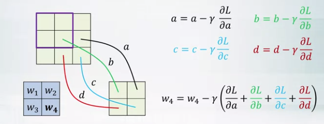
  • Gradients of the same shared weight are summed up.
• Convolutional vs fully connected layer
  • In convolutional layer, the same kernel is used for every output neuron. Share parameters of the network.
  • Fully connected layer where each output is a perceptron.
  • ex. 300x300 input, 300x300 output 5x5 kernel, convolutional layer needs 26parameters, \(8.1 x 10^9\) parameters needed in fully connected layer.
• A color image input
  • W X H X C tensor
• One convolutional layer is not enough
  • We use another convolutional layer above convolutional layer
  • In this case, Receptive for nth convolutional layer will be 2n+1 x 2n+1 when 1st convolutional layer cover 3x3.
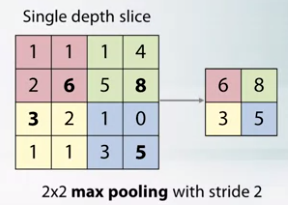
• Pooling layer
  • Works like a convolutional layer but doesn’t have kernel.
  • It calculates maximum or average of input patch values.
  • 
• Backpropagation for max pooling layer
  • Maximum is not a differentiable function.
  • No Gradient w.r.t to non maximum patch nuerons.
  • Change of maximum patch neurons will affect the output.

Modern CNNs

• Sigmoid activation
  • 
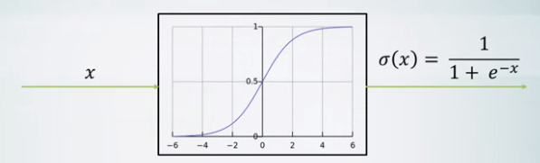
  • x for input and \(\frac {1} {1+e^{-x}}\) for output
  • If x is too small or too big, it can lead to vanishing gradients.
• Tanh activation
  • 
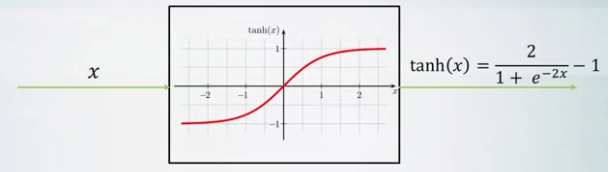
  • Zero-centered
  • Similar to sigmoid
• ReLU activation
  • 
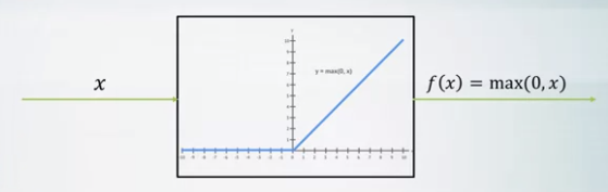
  • Fast to compute
  • Gradients do not vanish for positive x’s
  • Not zero centered
  • Can die when x initialized as less than zero
• Leaky ReLU activation
  • 
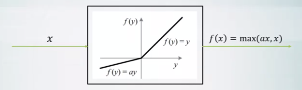
  • Will not die.
• Weights initializations
  • 
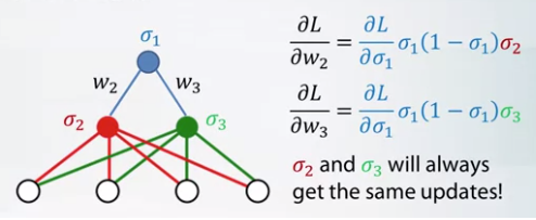
  • If we start with all zeros. simga 2 and sigma 3 have same updates.
  • We can break with small random numbers.
  • If we initialize like \(E(x_i) = E(w_i) = 0\) then the expected value of linear combination is zero.
  • 
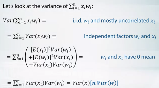
  • n Var(w) should be 1.
  • If it greater than 1, variance will increase while passing hidden layer.
• Batch normalization
  • normalize neuron output before activation
  • \(h_i = \gamma_i * \frac {h_i - \mu_i} {\sqrt {\sigma_i^2}} + \beta_i\).
  • \(\mu_i = \alpha * mean_{batch} + (1 - \alpha) * \mu_i\).
  • \(\sigma_i^2 = \alpha * variance_{batch} + (1 - \alpha) * \sigma_i^2\).
  • \(0 < \alpha < 1\).
  • Since normalization is a differentiable operation, we can apply backpropagation.
• Dropout
  • Reduce overfitting.
  • Keep neurons active with probability p.
  • During training, all nuerons are present but outputs are multiplied by p.
• Data augmentation
  • Since Datasets are not that huge, we apply flips, rotations, color shifts, scaling, etc.
• AlexNet(2012)
  • First deep CNN for ImageNet
  • 11x11, 5x5, 3x3 convolutions, max pooling, dropout, data augmentation, ReLU activations, SGD With momentum.
• VGG (2015)
  • Similar to AlexNet for using convolutions, pooling, etc.
  • only 3x3 convolutions but lots of filters.
• Inception V3 (2015)
  • Use Inception block.
  • Batch Normalization, image distrotions, RMSProp for gradient descent.
• 1x1 convolutions.
  • Capture interactions of input channels in one pixel of feature map.
  • Reduce the number of channel.
• Basic Inception block.
  • 
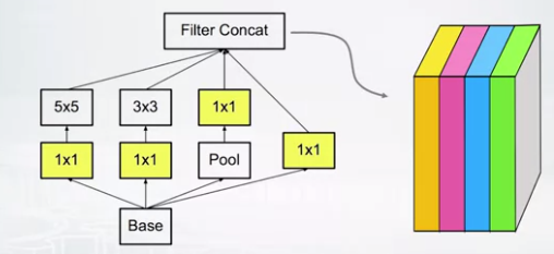
  • 4 different feature maps are concatenated on depth at the end.
  • We can replace 5x5 convolution to 2 3x3 convolutions.
• Filter decomposition in Inception block
  • 
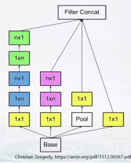
  • 3x3 convolutions are expensive parts.
  • Replace with 1x3 layer and 3x1 layer.
• ResNet (2015)
  • Introduces residual connections
  • few 7x7 convolution layers, rest are 3x3 convolution layers. batch normalization, max and average pooling.
• Residual connections
  • 
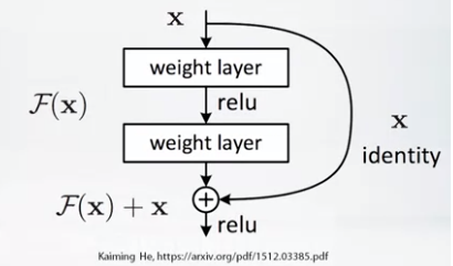
  • Create output channels adding a small delta F(x) to original input channels x
  • Can stack thousands of layers and gradients do not vanish.

Applications of CNNs

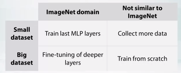
• Transfer learning
  • Deep networks learn complex features extractor, so we use it for a new task.
  • Less data to train
  • Can partially reuse ImageNet features extractor when domains are not realtive to ImageNet dataset. (ex. human emotions)
• Fine-tuning
  • Initialize deeper layers with values from ImageNet.
  • Don’t start with a random initialization.
  • Propagate gradients with smaller learning rate.

• 

• Semantic Segmentation
  • Need to classify each pixel
  • Pooling layer can’t be applied since it works as downsampling images.
  • 
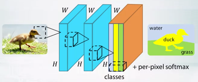
  • If we use pooling layer, we should upsample.
  • 
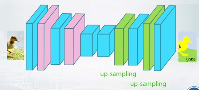
• Nearest neighbor upsampling
  • Fill with nearest neighbor values
  • get a pixelated values.
• Max unpooling
  • Remeber which element was max during pooling, and fill taht position during unpooling.
  • 
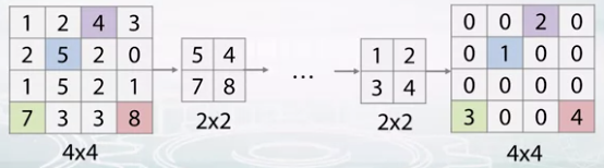
• Learnable unpooling
  • Replace max pooling layer with convolutional layer
• Object classification + localization
  • Find a bounding box of an object.
  • 
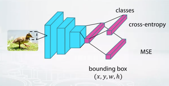
  • Train classification layer with cross-entropy
  • Reuse convolutional feature layer and train bounding box layer with MSE.
  • Loss will be the sum of 2 losses.