Advanced Machine Learning - Introduction to Deep Learning- Week1

This post is a summary for Advanced Machine Learning Course week1 in Coursera.

Before starting this lecture, You have to know below keywords.

• Linear Regression
• Logistic Regression
• Gradient Descent for Linear models
• Problem of overfitting
• Regularization for linear models

Linear model as the simplest neural network.

• Supervised Learning
  • \(x_i\) (example) : Image or Object we try to analyze in ML.
  • \(y_i\) (target value) : Ground truth or answer for image
• Regression and Classification
  • \(y_i \in \mathbb{R}\) : Regression
  • \(y_i\) belongs to a finite set : Classification
• Linear model for regression
  • \(y = b + w_1x_1 + w_2x_2 + ... + w_dx_d\).
  • \(w_i\) : coefficient (weights)
  • b : bias
  • d + 1 parameters (include b as \(w_0x_0 (w_0 = b, x_0 = 1)\) )
  • However, it’s hard to express with above formula.
    So we express with matrix, it can be expressed as \(a(x) = w^Tx\).
    If we apply it to all datasets(examples), it can be expressed as below.
    \(a(X) = Xw\)
    \(X = \begin{bmatrix} x_{11} & \dots & x_{1d} \\ \vdots & \ddots & \vdots \\ x_{l1} & \dots & x_{ld} \end{bmatrix}\)
• Loss function
  • Mesauring model quality.
  • Mean squared error : famous loss function
    • \(L(w) = \frac {1} {l} \sum_{i=1}^{l}(w^Tx_i-y_i)^2\) = \(\frac {1} {l} \parallel Xw - y \parallel ^2\).
  • Means how model fit to data.
• Training a model
  • Find w to minimize loss value.
• Summary
  • MSE used as a loss function in linear model
  • Exact solution exists, but it requires complicated operations.
• Linear model for classification
  • Multi-class classification problem
    • Can solve as K linear models and decide 1 class from these scores
• Classification loss
  • Classification accuracry : \(\frac {1} {l} \sum_{i=1}^{l}[a(x_i) = y_i]\)
  • [P] = Iversion bracket: if P is true return 1, if not return 0
  • Squared loss : \((w^Tx_i-1)^2\)
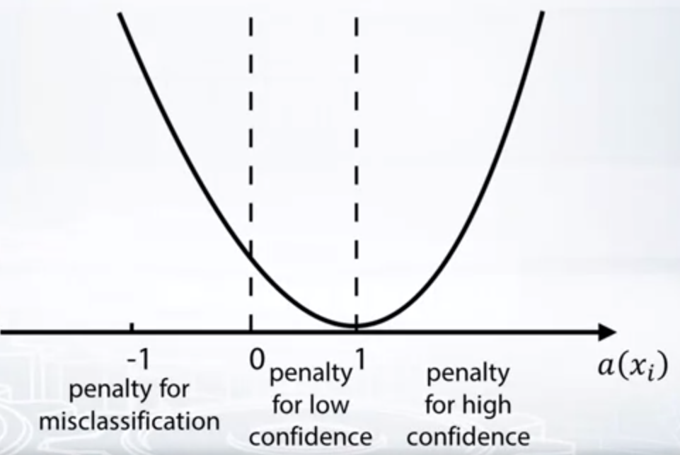
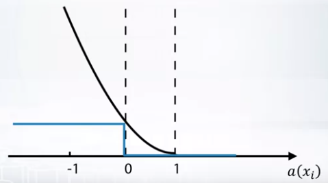
  • If we use squared loss, when our prediction is between 0 and 1, we penalize it for low confidence. If prediction is less than 0, we give large penalty. However when prediction is more than 1, it is weird to penalize due to high confidence. So we change the loss function as below.
    
• Class probabilites
  • softmax transform
    • convert scores from linear classifier to probabilites
    • \(\sigma(z) = (\frac {e^{z_1}} {\sum_{k=1}^{K}e^{z_k}}, ..., \frac {e^{z_K}} {\sum_{k=1}^{K}e^{z_k}})\).
• Cross-entropy
  • can be used as a loss function for classification
  • \(L(w, b) = -\sum_{i=1}^{l}\sum_{k=1}^{K}[y_i = k]log\frac {e^{w_j^Tx_i}} {\sum_{j=1}^{K}e^{w_j^Tx_i}}\).
• Gradient descent
  • To minimize value of loss function
  • the direction of the steepset slope at point.
  • \(w^0\) - initialization in some point
  • while True:
    \(w^t = w^{t-1} - \eta_t {\nabla}L(w^{t-1})\).
    if \(\parallel w^t-w^{t-1}\parallel <\epsilon\) then break
  • lots of heurisitcs:
    • How to initialize \(w^0\)
    • How to select step size \(\eta_t\)
    • When to stop
    • How to approximate gradient \({\nabla}L(w^{t-1})\)
• Gradient descent vs analytical solution
  • Graident descent is
  • easy to implement
  • can be applied to any differentiable loss function
  • require less memory

Regularization in machine learning

• Overfitting example
  • 
    
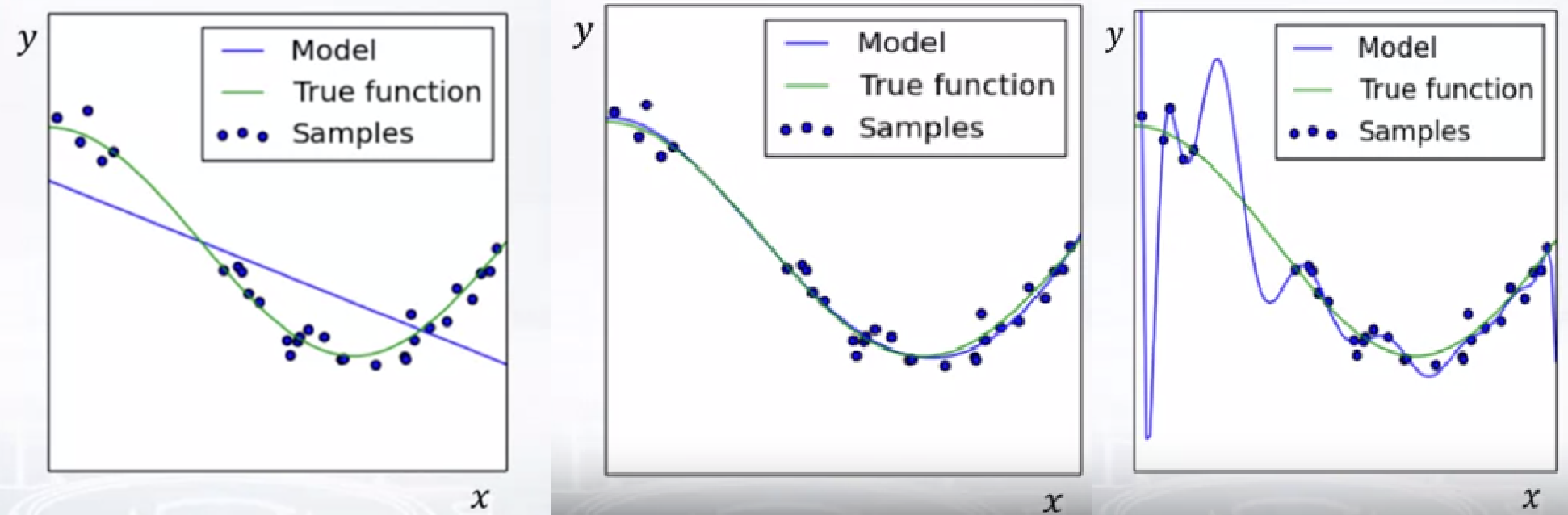
  • To overcome fitting the model properly to real data, linear model can’t predict value well as 1st picture. However, 3rd picture shows model which is overfitted to our data. It’ll show poor performance on new datas.
• Overfitting example2
  • 
    
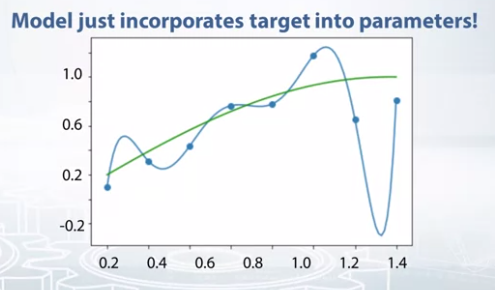
  • Training set for above picture is {0.2, 0.4, … 1.6} and target value for them are \(sin(x) + \epsilon\)
  • However, model with degree 8 get 0 for loss function when parameters are (130.0, -525.0, …)
  • In this case, range of target value are 0 to 1 but parameters are more than 100.
• Holdout set
  • For valiating our model, we divide to training set and holdout(validation) set.
  • 7:3 ~ 8:2
  • If dataset is small, we use cross-validation
  • 
    
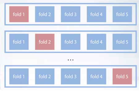
  • Cross-validation trains K times for K-fold
• Regularization
  • Overfitting model have large weights, good model have not ver large weight
  • For it, we modify the loss function
• Weight penalty
  • \(L_{reg}(w) = L(w) + \lambda R(w)\).
    • L(w) : loss function
    • R(w) : regularizer (penalizes large weights)
    • \(\lambda\) : regularization strength
• L2 penalty
  • We can use L2 penalty as weight penalty
  • \(L_{reg}(w) = L(w) + \lambda \parallel w \parallel^2\).
  • \(\parallel w \parallel^2 = \sum_{j=1}^{d} {w_j}^2\).
  • drives all weights closer to 0
• L1 penalty
  • \(L_{reg}(w) = L(w) + \lambda \parallel w \parallel_1\).
  • \(\parallel w\parallel_1 = \sum_{j=1}^{d} \mid{w_j}\mid\).
  • Drives some weights exactly to 0
  • Depends only on some features.
• Other regularization techniques
  • Dimensionality reduction
  • Data Augmentation
  • Dropout
  • Early Stopping
  • Collect more data

Stochastic methods for optimization

• Gradient descent
  • we start with \(w_0\) and calculate with gradient.
  • However, if we use MSE, we should sum gradients of all examples. It’ll make too many calculations.
• Stochastic gradient descent
  • To overcome the problem above, we use stochastic gradient descent.
  • At every step, we select reandom examples of our dataset and calculate gradient with only that example.
  • It lead noisy approximation.
  • need only one example on each step, so can be used in online learning.
  • learning rate \(\eta_t\) should be chosen carefully.
• Mini-batch gradient descent
  • We choose m examples and calculate gradient with these examples.
  • still learning rate \(\eta_t\) should be chosen carefully.
• Difficult function
  • 
    
  • Gradient descent will oscillate and iterates many time.
• Momentum
  • \(h_t = \alpha h_{t-1}+\eta _tg_t\).
  • \(w^t = w^{t-1}-h_t\).
  • Tends to move in the same direction as on previous steps.
  • reduces oscillation of gradient descent
• Nesterov momentum
  • \(h_t = \alpha h_{t-1} + \eta _t {\nabla}L(w^{t-1}-\alpha h_{t-1})\).
  • \(w^t=w^{t-1}-h_t\).
  • converged well than momentum
  • still have to choose learning rate
• AdaGrad
  • choose learning rate adaptively
  • \(G_j^t=G_j^{t-1}+g_{tj}^2\).
  • \(w_j^t=w_j^{t-1}-\frac {\eta _t} {\sqrt {G_j^t + \epsilon}} g_{tj}\).
  • don’t need to choose learning rate wisely
• RMSprop
  • \(G_j^t = \alpha G_j^{t-1} + (1-\alpha)g_{tj}^2\).
  • \(w_j^t = w_j^{t-1} - \frac {\eta _t} {\sqrt{G_j^t + \epsilon}}g_{tj}\).
  • overcome the problemn of large sums of square gradients
  • depends only on last examples from gradient descent method.
• Adam
  • \(m_j^t=\frac{\beta _1m_j^{t-1}+(1-\beta _1)g_{tj}} {1-\beta _1^t}\).
  • \(v_j^t=\frac{\beta _2v_j^{t-1}+(1-\beta _2)g_{tj}^2} {1-\beta _2^t}\).
  • \(w_j^t=w_j^{t-1}-\frac{\eta _t} {\sqrt{v_j^t} + \epsilon}m_j^t\).